How to Make School Result in Excel Worksheet?
Nowadays almost every institution is computerized. They are using Computers for almost everything like Fee receipts, School Results, etc. For making School Result in Excel. You have to first open Excel on Your Computer or Laptop.
Just type Excel in your Start Menu search, you will get MS Excel. After Opening MS Excel successfully.
Write the School Name on the top row and Merge and Centre the number of Columns you want for Your School name. You can try yourself, for the best look you want for your Excel Sheet.
Write the Roll Numbers, Names, Subject Marks in the Excel Sheet with Total Column, Percentage Column, and Result i.e., Pass or Fail Column.
Add Names and Marks of the students. For convenience, we have used 3 subjects.
https://youtu.be/C2YAo-StBao
How to Calculate Total Marks in Excel Workbook?
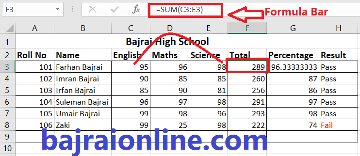
Now, here we have to calculate the total marks of the students on the Excel Sheet. Calculating Total in Excel is very easy, just type is equal to sign (“=”) and write “SUM”, open the Bracket and select the Cell of First Subject Marks of the student. In Our Case, it C3, then type colon symbol “:” and select the last subject cell. In our case it is c5, now close the bracket and click enter.

The formula for Calculating Total / Total Marks in Excel Workbook
=SUM(C3:C5)
Hurray! You have calculated the total number of marks students obtained in the exam.
Note: if you have 10 subjects or more you have to just select the last subject cell after colon and You will get the total.

How to Calculate the Percentage of Marks in Excel Worksheet?
For calculating Percentage or Student Percentage in Excel Workbook, just you have to write an easy formula.
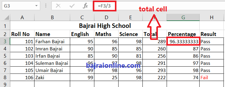
Type “=” in the percentage cell and then type total marks cell divided by a number of subjects.
In our case it is the total marks cell is F3, and the total number of subjects is 3.
Student Percentage Formula in Excel Worksheet
=F3/3
F3 is the total marks cell and 3 is the number of subjects.
In this formula, we come across a small issue, that if the percentage is in decimal, then it will show in decimal only. In our case, it is showing 96.33. We don’t want to show percentage in decimal, rather we want to roundup this and show only integer value. No need to panic, we have the formula to overcome this problem.
How to Roundup Student Percentage in Excel?
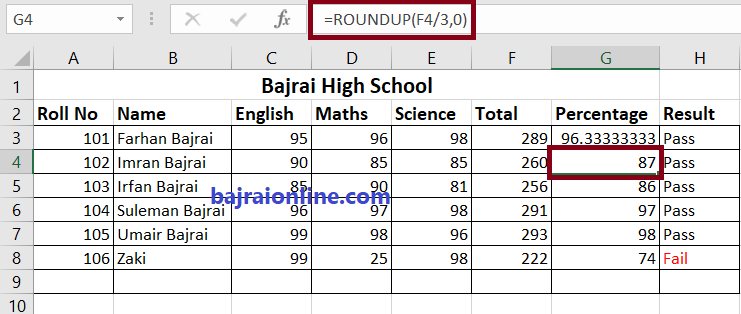
To round up student percentage in Excel Workbook. Just You have to use ROUNDUP formula. Just type ROUNDUP after = sign in the percentage cell, then open the bracket and write percentage formula, in our case it is F4/3. After this, just type comma “,” and then ZERO “0” and close the Bracket.

Congrats! You have successfully displayed the Student’s Percentage marks in Excel Without decimal value.
ROUNDUP FORMULA in Excel
=ROUNDUP(F3/3,0)

How to Display Result (Pass or Fail) in MS Excel?
After calculating the total marks, percentage of students successfully, now you have to show whether he/she is pass or fail. For this, we have to check each and every subject’s mark. Because maybe a Student has a good percentage and he/she is failed in any subject. Normally, we have 35 marks to pass in a subject.
For checking pass or fail, we have to use logical formula i.e., the IF formula in Excel.
For checking each subject mark, we need to use AND formula. So here we have to use two formulas at a time. Let use them.
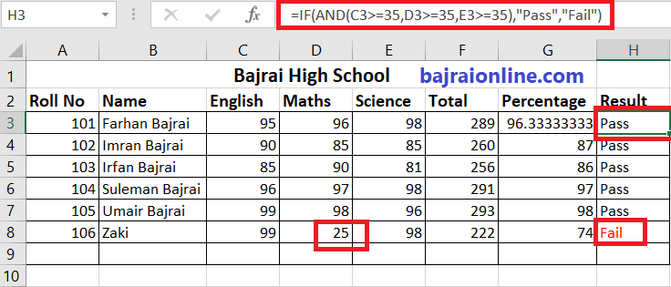
In Result Cell, after “=” type IF and open the bracket. After Bracket type AND, then open one more bracket. Now you have to check each and every subject’s marks, it should be greater than equal to 35. The first subject mark is in C3. We should write C3>=35, after that use comma and write a second cell condition, in our case it is D3>=35. Then last subject E3>=35. After checking marks of all subjects close the bracket and write comma “,” after it. Now, Write in double quotes “PASS” then write comma “,” and Write in double quotes “FAIL”. At the end Close the Bracket. Now click enter.
Yay! You have successfully displayed PASS or FAIL results in Excel Sheet.
Pass/Fail Formula in Excel Worksheet?
=IF(AND(C3>=35,D3>=35,E3>=35),”Pass”,”Fail”)
Note: Be careful while writing the formula, we are opening and closing 2 brackets in this formula. One bracket is opening after if and it is closing after the last subject condition check. And the other bracket is opening after AND, it is closing in the last. If you miss any bracket or comma or quotes, then you will get the error.
So by this, you have successfully displayed the school result in Excel WorkBook. Do comments, for any queries.
